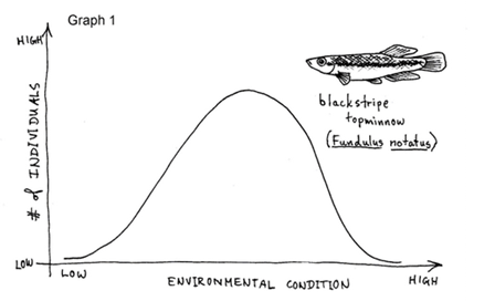
Tolerance Range

TOLERANCE RANGE

Biologists are frequently interested in studying and understanding the tolerance ranges of different species for different environmental factors. If you draw a graph of how many individuals in a population live under which part of the range of any given factor, you almost always get a bell-shaped curve. Take a look at the two tolerance range curves shown below. The horizontal axis could be any of the abiotic factors (environmental conditions), but for now let’s say it is for oxygen levels in freshwater lakes. If you are studying a particular species of fish, let’s say the blackstripe topminnow (Fundulus notatus), you could go out and measure the oxygen level of every lake where you find the topminnow and also count how many topminnows are in each lake. When you make a graph of your data, it might look like Graph 1. That graph is telling you that the majority of the topminnows live in the middle part of the oxygen range; that’s where the curve is highest. As you move from the middle part to lower oxygen levels (to the left) or to higher oxygen levels (to the right), the curve is not as high – there are fewer individuals that live in lakes that have the lower or higher amounts of oxygen. And if the oxygen level is extremely low or high, it is beyond the tolerance range of the species and no topminnows live in those lakes.

Now take a look at Graph 2, which represents the oxygen tolerance range curve for a different species of fish, in this case the blacktail shiner (Cyprinella venusta).

What is Graph 2 telling us about shiners compared to the topminnows? Shiners have a much narrower tolerance range for oxygen than topminnows do. The shiner can only survive and thrive in a narrow band of oxygen levels, so you would expect that its geographical range would be more restricted; it would not be distributed as widely as the topminnow since it wouldn’t do well in stagnant ponds with lower oxygen levels, for example. If you look closely, you’ll also notice that the peak of the curve for the shiner is a little bit to the right of the peak of the curve for the topminnow. This tells us that compared to topminnows, shiners do best in water that is slightly more oxygenated.

Both Graph 1 and Graph 2 are bell-shaped curves. That’s the normal or typical curve you get when graphing tolerance ranges, and interestingly enough, curves shaped like this illustrate what is referred to as a normal distribution. In some ways, you could say it is the "Goldilocks curve" – it shows where conditions are just right for a species: not too hot, not too cold; not too salty, or not salty enough; not too wet, not too dry. These preferences and needs for certain types of conditions greatly influence the distribution of species around the planet, and it can get fairly complex when you consider that multiple abiotic factors are simultaneously influencing any given individual and species.